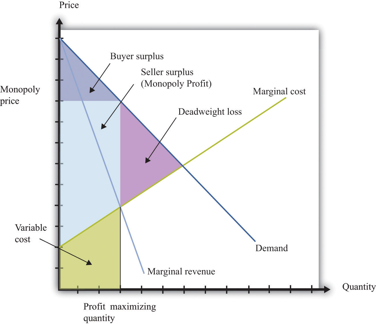
In the case of pure monopoly, the firm and the industry coincide by definition. The output of the monopolistic firm should, therefore, be compared with that of the industry under perfect competition; Fig. 14.1 compares the demand supply analysis of the competitive industry with the marginal apparatus of the theory of the firm.
We show profits (or losses) as the case may be in Fig. 14.1, where the marginal cost (MC) curve is U-shaped. In this figure, MC curve lies above MR curve up to OQo level of output. Every unit of output produced in this range, thus, adds more to the cost than to the revenue.
That is why, point E cannot be the point of equilibrium, where MC curve cuts MR curve from above. Rather, at this point, the firm invariably obtains the net loss (negative profit), shown by heavily shaded area DBE in Fig. 14.1. A move in either direction from point ‘E ‘ will help the firm either by reducing its costs more than it cuts its revenue (a move to the right) or by adding to its revenue more than to its cost (a move to the left).
ADVERTISEMENTS:
There is an incentive for the firm to continue production, since; marginal revenue exceeds marginal cost beyond point Eq. Hence, MC-MR equality (i.e., where marginal profit is zero) is merely a necessary condition, but, not sufficient condition for equilibrium.
For every additional unit produced beyond point E0, the firm can add to its profit by the excess of the marginal revenue over marginal cost, until marginal revenue (MR) and marginal cost (MC) are once again equalised at point ‘E’. After remaining below the MR curve, MC curve cuts the former from below at the equilibrium point ‘E’.
ADVERTISEMENTS:
With this, the second order condition (necessary condition) that slopes of MR curve should be less than that of MC curve is also satisfied. At equilibrium, the output produced is OQ. The firm has no incentive to produce beyond OQ level of output; as such attempt would only reduce the total profits of the monopolist.
At equilibrium point ‘E’, total profit (which is the difference between total revenue and total cost) is given by the lightly shaded area between points E0 and ‘E’ minus the heavily shaded area DBE0, i.e., area under the MR curve minus area under the MC curve up to equilibrium point ‘E’.
Stopping production before OQ level of output would reduce the profit area, shown by the lightly shaded area. While production of additional units beyond OQ level of output would add more to the cost than to the revenue, thereby reducing the total profit. Hence, only point ‘E’ is the point of equilibrium, where both the equilibrium conditions are satisfied. A small increase or decrease in quantity will reduce the total profit.
Given average cost curve, it is also possible to show net profit (or loss) as the case may be in terms of the area of a rectangle. Such representation is now explained both for the short-run and long- run. As a monopolist is the only producer, there is no need to have a separate theory of the firm and the industry, as is necessary under perfect competition.

