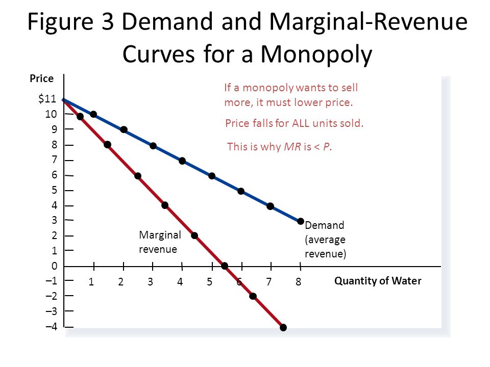
Relationship between “Average Revenue Curves” and “Marginal Revenue Curves”

Relationship between “Average Revenue Curves” and “Marginal Revenue Curves” are described below:

If both AR and MR curves are straight lines, it can be shown that MR curve is half-way from the AR curve on the Y-axis. Consider Fig. 12.2 in which we have straight line AR and MR curves. A point ‘P’ is taken on the Y-axis and a line PS is drawn parallel to the X-axis.

The line PS cuts the MR curve at point ‘R’. To show that MR cuts the distance between Y-axis and the AR curve in the middle implies that in Fig. 12.2, PR = RS.

Image Source: images.slideplayer.com

Now, from point ‘S’ draws a line SQ perpendicular to the X-axis. We can find the TR received by the seller from the sale of OS unit of the commodity in two ways.

Because all the three angles of the two triangles are equal to each other, the two triangles ASR and BPR are similar.

It is proved that both the triangles are equal in area and similar too. Thus, they must be congru­ent. If two triangles are congruent, their corresponding sides are equal. It means that

PR = RS

Hence, if AR and MR curves are straight lines, then, MR curve bisects the distance between the Y-axis and the AR curve. This relationship between the AR and MR curves can be used in drawing the two curves. But, this relationship between AR and MR curves is not true, if the two curves are either convex or concave to the origin.

As shown in Fig. 12.3 (a), if, AR and MR curves are convex to the origin, MR cuts the distance between the Y-axis and AR at less than half-way as measured from the Y-axis (i.e., to the left of the middle point). And, if, the AR and MR curves are concave to the origin, MR curve cuts the distance between the Y-axis and AR at more than half- way as measured from the Y-axis (see Fig. 12.3 (b)). In either of the two cases, MR curve will not lie half way from the Y-axis. The proof of this is beyond the scope of this book.

But, AQ is marginal revenue and SQ is average revenue corresponding to point ‘B’ at OQ level of output. Hence, equation (12.7) can be written as

The above relationship can be utilised to find out the marginal revenue corresponding to the average revenue at any given level of quantity sold, provided the price elasticity of demand is known.

The relation between AR, MR and elasticity of demand (e) can now be written as

With the help of the above formula, it is possible to find MR, given AR (price) and elasticity of demand. For example, for AR =10 and e = 2,

Thus, for e – I, MR = 0. This is very useful relationship and should be noted carefully. Here, total revenue (outlay) is not affected by change in price as discussed under total outlay method in Chapter 4 on Elasticity of Demand.

It can also be shown that at every point on the demand curve, where elasticity is greater than unity, MR is positive (but, less than AR). Further, at every point on the demand curve where elasticity is less than unity, MR is negative.

This can be verified by substituting the value of elasticity in equation (12.9). An increase in the price will result in an increase and a decrease of the total revenue in these two cases respectively and vice-versa. AR, being price is always positive.

In Fig. 12.5, elasticity at middle point ‘S’ is SB/SB, i.e., 1 and MR is equal to zero. MR curve is shown cutting the X-axis at point ‘Q’. At all the points on the demand curve between ‘S’ and ‘B’ (for a lesser quantity than OQ), the numerator is greater than the denominator. Hence, e > 1 and MR is positive. Further, at all the points on the demand curve between ‘S’ and ‘C’ (for a greater quantity than OQ) numerator point is less than the denominator. So, e < 1 and MR is negative.

In extreme case, when the elasticity of demand is zero, AR is equal to zero while MR is equal to minus infinity and so the gap between the two is maximum. When the elasticity of demand increases to 1/3, MR becomes AR ((1/3 – 1) / 1/3) or (-2AR).

With further increase in the value of the elasticity of demand to 1/2, MR becomes AR ((1/2 – 1) / 1/2) or (-AR). When the elasticity of demand rises to 2, MR becomes AR ((2 – 1) / 2) = AR/2. With further rise in the value of elasticity of demand to 3, MR becomes AR ((3 – 1) / 3) = 2 / 3 AR In other extreme situation, when the elasticity of demand is infinity, MR is equal to AR.

Thus, we observe that as the value of elasticity of demand increases, MR and AR curves become closer and closer to each other. The gap between them reduces to zero under perfect competition, when the demand curve is perfectly elastic.