How Long Run Marginal Cost Curve is Derived from the Short Run Marginal Cost Curves?

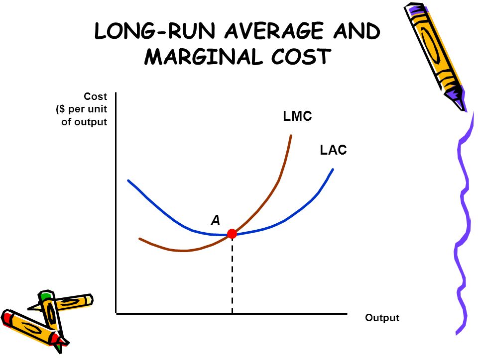
The long run marginal cost (LMC) curve shows the minimum amount by which cost is in­creased each time, when output is increased or the maximum amount of total cost that can be reduced, when output is reduced.

LMC curve is derived from the short run marginal cost (SMC) curves by considering the points of intersection of the SMCs, with vertical lines drawn from the points of tangency of corresponding SAC and LAC curve to the X-axis. This is illustrated in Fig. 9.14, where initially LAC curve is drawn through short- run average cost (SAC) curves. For the sake of simplicity, only three SAC curves have been considered.

In the long run, if the firm wants to produce OQ, output, it will choose the plant corre­sponding to SAC₁. For this level of output, LAC curve is tangent to SAC, at point ‘A’. The corresponding LMC will be equal to SMC₁ (i.e., BQ₁) at point ‘B’ corresponding to OQ₁ level of output. This happens, because, where for a given level of output, LAC is equal to SAC₁ the LMC will also be equal to SMC.

Image Source: images.slideplayer.com

Thus, the LMC curve passes through point ‘B’. Further, if OQ₂ output is produced, the firm will choose the plant corresponding to SAC₂. For this level of output, ‘E’ is the point on LAC curve, where both SAC₂ and SMC₂ are equal, as the former attains minimum value at this point.

Therefore, for OQ₂ level of output, LMC is equal to SMC₂. The LMC curve will thus, pass through point ‘E’. This implies that the production of output level of OQ, in the long run involves marginal cost of EQ₂.

Finally, for output level of OQ₃, the LMC is equal to SMC₃ corresponding to the point of tangency between LAC and SAC₃ at point ‘C’. The SMC₃ corresponding to this point (or OQ₃ level of output) is given by point ‘D’. This is the point through which LMC curve will pass. LMC for OQ₃ level of output is equal to DQ₃.

Fig. 9.14: Long Run Marginal Cost Curve

The LMC curve is derived by joining points ‘B’.’E’ and ‘D’. This curve passes through those points of SMCs, which correspond to respective tangency points of short run average cost curves with LAC curve.

The LMC curve can be defined as the locus of those points on the SMC curves, which correspond to the optimum plant size (and not the optimum output, i.e., the points of minimum SACs) for each output

The LMC can also be constructed by plotting the derivative of long-run total cost with respect to output level. In any case, the LMC is not the envelope of the short run marginal cost curves. Therefore, portions of SMC curves may lie below the LMC curve.

In other words, the short and the long run marginal cost curves may cross. Further, the LMC curve is flatter than the short-run marginal cost curve as (i) the U shape of the LAC curve is less pronounced than that of the SAC curve, and (ii) marginal costs rise more sharply in short run than in the long run.